0%

因果推断 | 倾向得分匹配(PSM)// Propensity Score Matching

倾向评分匹配

倾向评分匹配/倾向性得分匹配(PSM,Propensity Score Matching)

  • 通过观测变量对实验组的预测概率进行匹配
  • 处理观察性研究(observational study)的经典方法
  • 可以解决内生性问题

适用情形:

  1. 在观察研究中,对照组与实验组中可直接比较的个体数量很少
  2. 由于衡量个体特征的参数很多,所以想从对照组中选出一个跟实验组在各项参数上都相同或相近的子集作对比变得非常困难
  3. 对照组和实验组之间的差异可能是选择性偏差导致的,不一定是干预策略导致的

Why Propensity Score Matching?

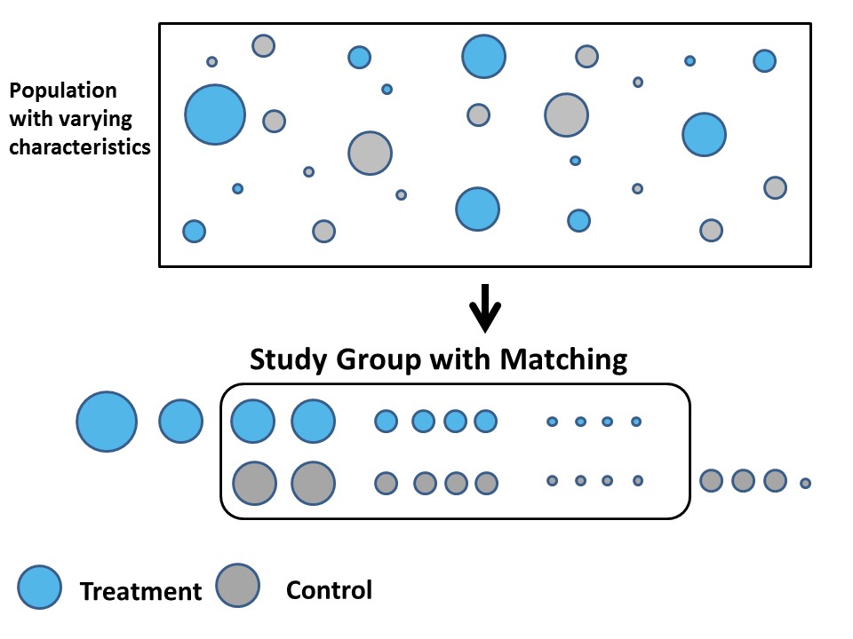
Picture from PROPENSITY SCORE MATCHING(PSM图解)

倾向性得分:一个用户/样本属于实验组的“倾向性”(给定$x$的情况下,样本进入实验组的条件概率)。
$$e(x)=P\left(T=1|X=x\right)$$
其中,

  • $T$:干预
  • $X$:样本属性/协变量
  • $Y$:观测结果/结果变量

Theorem 1: 平衡性质(Balancing Property):
$$T_i \perp X_i \mid e(X_i)$$

Theorem 2: 无混淆(Unconfoundedness)
$$ T_i \perp Y_{i0}, Y_{i1} \mid e(X_i)$$

  • 倾向性得分是一种“Balancing score”
  • 对于倾向性得分$e(X_i)$相同的一群用户$i$:
    • 干预$T_i$和特征$X_i$是独立的
    • 干预$T_i$和潜在结果$Y_{i0}, Y_{i1} $是独立的
  • 当协变量$X$不影响干预变量$T$、但影响结果变量$Y$时,引入协变量可以提高干预精度
  • 当遗漏了重要的协变量时,会导致偏差

前提/假设

PSM需满足以下两个前提/假设:

  1. 条件独立假设:控制了协变量后,样本是否接收干预与潜在结果相互独立
  2. 共同支撑条件:若匹配结果较为理想,匹配后的两条核密度曲线较为相近

匹配方法

PSM通过统计模型对每个样本计算倾向性得分,再按照倾向得分是否接近进行匹配。
以分组变量为解释变量(分类变量),样本属性(可能会影响到结果的变量)作为被解释变量,进行逻辑回归(Logistic Regression),从而计算每个样本的倾向性得分。

  • 一对一匹配:在控制组中选择与实验组样本最相近的单个样本进行匹配
    • 优点:匹配的样本之间较为相近,偏差较小
    • 缺点:样本匹配量小、估计的方差较大
  • 一对多匹配:在控制组中选择多个与实验组样本相近的样本进行匹配
    • 缺点:在控制组中找到的第2个、第3个、……样本与实验组样本的近似性会减弱,会增大估计的偏差

控制组样本量较多时,可以考虑使用一对多匹配

匹配方法 特点 偏差 方差
最近邻匹配 增加近邻数,可重复使用
半径匹配 容忍度增加
核匹配 带宽增加
卡尺匹配 容忍度增加
分块匹配法

最近邻匹配

最近邻匹配(Nearest-neighbor Matching):选择控制组中倾向性得分最接近的样本作为匹配样本

干预样本$i$与无干预样本$j$相匹配:
$$
\begin{equation}
\mid p_i - p_j \mid = \min_{k \in { T=0 } } \left\lbrace \mid p_i - p_k \mid \right\rbrace
\end{equation}
$$

半径匹配

半径匹配(Radius Matching):

核匹配

核匹配(Kernel Matching)

卡尺匹配

卡尺匹配(Caliper Matching):给定误差 $\delta > 0$,干预样本$i$与无干预样本$j$相匹配
$$
\begin{equation}
\delta > \mid p_i - p_j \mid = \min_{k\in { T=0 } } \left\lbrace \mid p_i - p_k \mid \right\rbrace
\end{equation}
$$

  • 可能会有样本找不到匹配对象

分块匹配法

分块匹配法(Stratification)

匹配效果检验

应用因果推断方法尽可能保证干预组与控制组的分布较为相近(尽可能在已观测到的变量上同质),尽可能去“模拟”随机试验的情况,需要结合一定检验方法来检验“模拟”效果,以保障因果推断评估结果的稳健性(Robust)。

共同支撑检验

共同支撑检验(Common Support Test):为了提高匹配质量,仅保留倾向得分重叠部分的个体(会损失一定的样本量)。

方法:

  • 比较匹配前后的核密度图
  • 绘制条形图,显示倾向得分的共同取值范围

平衡性检验

平衡性检验(Balance Diagnose):观察匹配后的各个变量的均值是否有显著差异。计算每个变量的干预组和虚拟控制组的差异(SMD,Standardized Mean Difference)。

$$
\begin{equation}
\mathrm{ SMD } = \frac{ \bar{ X }{ \mathrm{ Treat } } - \bar{ X }{ \mathrm{ Control } } }{ \sqrt{ \frac{1}{2} \left( s^2_{ \mathrm{ Treat } } + s^2_{ \mathrm{ Control } } \right) } }
\end{equation}
$$

  • 相关论文:Zhang, Z., Kim, H. J., Lonjon, G., & Zhu, Y. (2019). Balance diagnostics after propensity score matching. Annals of translational medicine, 7(1).
  • 经验表明,如果一个变量的SMD不超过0.1,一般认为这个变量的匹配质量可以接受;否则,需要结合经验来判断该变量是否可以剔除。

反驳式检验

反驳式检验(Refute):

  • 添加随机混杂因子:添加随机的混杂因子(控制特征),如果因果效应变化较小,表明PSM结果较为稳健
  • 安慰剂检验:将干预替换为随机变量,如果因果效应接近于0,表明PSM结果较为稳健

反驳式检验本质上是弱检验,检验通过表明PSM估计结果在已有的控制变量上能够保持较好的稳健性;检验不通过,则认为PSM估计结果是不可用的,需要重新评估。

敏感性分析

敏感性分析(Sensitivity Analysis):TBD

Pros & Cons

优势 Strengths

  • 在计算倾向性得分时,考虑了交互项(interaction terms)
  • 可用于二分变量(dichotomous variables)和连续变量(continuous variables)
  • 较少依赖于p值或其他特定于模型的假设

局限性 Limitations

  • 需要大样本(PSA works best in large samples to obtain a good balance of covariates.)
  • 要求控制组和实验组有较大的共同取值范围(Group overlap must be substantial to enable appropriate matching.)
  • 要尽可能控制可观测的变量,如果存在不可观测的协变量,会导致“隐形偏差”(The most serious limitation is that PSA only controls for measured covariates. Matching on observed covariates may open backdoor paths in unobserved covariates and exacerbate hidden bias.)
  • 没有考虑样本的聚集性,邻域层级的研究可能会存在问题(Does not take into account clustering (problematic for neighborhood-level research).)

Python

pymatch

causalinference

DoWhy

相关资料:

实例

伪Demo(pymatch)

1
2
3
4
5
6
7
8
9
10
11
12
13
14
15
16
17
18
19
20
21
22
23
24
25
26
27
28
29
30
31
32
33
34
35
36
37
38
39
40
41
42
43
44
45
46
47
48
49
50
51
52
53
54
55
56
57
58
59
60
61
62
63
64
65
66
67
68
69
70
71
72
73
74
75
76
77
78
79
80
81
82
83
84
85
86
87
88
89
90
91
92
93
94
95
96
97
98
99
100
101
102
103
104
105
106
107
108
109
110
111
112
113
114
115
116
117
118
119
120
121
122
123
124
125
126
127
128
129
130
131
132
133
134
135
136
137
138
139
140
141
142
143
144
145
146
147
148
149
150
151
152
153
154
155
156
157
158
159
160
161
162
163
164
165
166
167
168
169
170
171
172
173
174
175
176
177
178
179
180
181
182
183
184
185
186
187
188
189
190
191
192
193
194
195
196
197
# 载入需要的库
import pandas as pd
import numpy as np
import os

import warnings
warnings.filterwarnings('ignore')

from pymatch.Matcher import Matcher
from causalinference.causal import CausalModel

from xgboost import XGBClassifier, plot_importance
from sklearn.model_selection import train_test_split
from sklearn.metrics import roc_auc_score, accuracy_score, precision_score, recall_score, f1_score
from scipy import stats
from statsmodels.stats.power import GofChisquarePower
from statsmodels.stats.proportion import proportion_effectsize as es

import matplotlib.pyplot as plt
from IPython.display import display

# 自定义检验函数
def chi2_test(df1, df2, col):
'''
卡方检验
'''
n_table = [] ## 存储列联表
## 待检验指标的类别枚举值
vals1 = set(df1[col].unique())
vals2 = set(df2[col].unique())
col_values = set(vals1 + vals2)

for val in col_values:
if val in vals1:
a = len(df1[df1[col] == val])
else:
a = 0
if val in vals2:
b = len(df2[df2[col] == val])
else:
b = 0

n_table.append([a, b])

stat, pval, d_f, expected = stats.chi2_contingency(n_table)
return pval

def continuous_test(df1, df2, col):
'''
连续指标的显著性检验
'''
result = []

if len(df1[col]) < 30 or len(df2[col]) < 30:
result = [-1.0, '样本量过少']
else:
## 1. 正态性检验
norm_stat1, norm_pval1 = stats.kstest(df1[col], 'norm')
norm_stat2, norm_pval2 = stats.kstest(df2[col], 'norm')
if norm_pval1 > 0.05 and norm_pval2 > 0.05:
## 正态性检验通过
## 2.1 方差齐性检验
F = df1[col].var() / df2[col].var()
n1 = len(df1[col]) - 1
n2 = len(df2[col]) - 1
F_pval = 1 - stats.f.cdf(F, n1, n2)
if F_pval < 0.05:
## 方差齐性检验不通过
## 3.1 不等方差T检验(Welch T Test)
stat, pval = stats.ttest_ind(df1[col], df2[col], equal_var=False)
test_method = 'Welch-t检验'
else:
## 方差齐性检验通过
## 3.2 等方差T检验(Student T Test)
stat, pval = stats.ttest_ind(df1[col], df2[col], equal_var=True)
test_method = 'Student-t检验'
else:
## 2.2 MWU非参数检验
stat, pval = stats.mannwhitneyu(df1[col], df2[col], alternative='two-sided')
test_method = 'Mann-Whitney-U检验'
result = [pval, test_method]
return result

# 数据准备
df = pd.read_csv("xxx.csv", encoding='utf_8_sig')
df.head()

len(df)

## 一些数据处理
## 1. 缺失值填补
cols_fn0 = [
## 一些需要用0填补缺失值的列名
]
for col in cols_fn0:
df[col] = df[col].fillna(0)

## 2. 剔除多余的列
cols_drop = [
## 需要剔除的列
]
df = df.drop(cols_drop, axis=1)

# 特征重要性(筛选变量)
cols_x = [
## 特征
]

cols_y = [
## 因变量
]

X = df[cols_x]
y = df[cols_y]
## 如果特征的量纲较大,应先进行标准化
arr_mean = np.mean(X)
arr_std = np.std(X, ddof=1)
newX = (X - arr_mean) / arr_std
X = newX

print("XGBoost Start!")
# 训练模型
model = XGBoostClassifier()
model.fit(X, y)

df_ip = pd.DataFrame(columns=['Feature', 'Importance'])
df_ip['Feature'] = X.columns
df_ip['Importance'] = model.feature_importances_
df_ip = df_ip.sort_values(by=['Importance'], ascending=False)
df_ip = df_ip.reset_index(dro=p=True)
df_ip.to_csv('xxxxx_xgboost_feature_importance.csv', index=False, encoding='utf_8_sig')

cols_ip = df_ip.Feature[:10].to_list() ## 选取TOP 10特征最为PSM的控制特征
display(df_ip)
print("XGBoost Done!\n")

cols_cate = [
## Category特征
]
for col in cols_cate:
if col in cols_ip:
df[col] = df[col].astype('category')

# PSM
print("PSM Start!")
df1 = df[cols_ip + ['new_index', 'group_name']]
experiment = df1[df1.group_name == 'experiment'].reset_index(drop=True)
control = df1[df1.group_name == 'control'].reset_index(drop=True)

experiment['treatment'] = 1
control['treatment'] = 0

cols_exclude = [
## 不参与PSM的特征
]
m = Matcher(experiment, control, yvar='treatment', exclude=cols_exclude)

np.random.seed(2022) ## 设置随机seed,以便后续结果能够复现
m.fit_scores(balance=True, nmodels=100)
print("1. Fit Scores Done!")

m.predict_scores()
fig = plt.figure(figsize=(10, 5), dpi=200)
m.plot_scores()
fig.savefig('xxx_PSM_scores_plot.jpg')
print("2. Scores Plot Done!")

fig = plt.figure(figsize=(10, 5), dpi=200)
m.tune_threshold(method='random')
fig.savefig('xxx_PSM_tune_threshold_plot.jpg')
print("3. Tune Threshold Plot Done!")

m.match(method='min', nmatches=1, threshold=0.0001)
print("4. Match Done!")

df_freq = m.record_frequency()
df_freq.to_csv('xxx_PSM_record_frequency.csv', index=False, encoding='utf_8_sig')
print("5. Record Frequency Done!")

df_matched = m.matched_data.sort_values('match_id') ## 匹配后的数据
df_matched.to_csv('xxx_PSM_matched_data.csv', index=False, encoding='utf_8_sig')
print("6. Matched Data Saving Done!")

df_original = m.data ## 源数据(含scores)
df_original.to_csv('xxx_PSM_original_data.csv', index=False, encoding='utf_8_sig')
print("7. Original Data Saving Done!")

if len(set(cols_cate).intersection(set(cols_ip))) < len(cols_ip):
cc_continuous = m.compare_continuous(return_table=True)
cc_continuous.to_csv('xxx_PSM_compare_continuous.csv', index=False, encoding='utf_8_sig')
print("8.1 Compare Continuous Done!")
elif len(set(cols_cate).intersection(set(cols_ip))) > 0:
cc_categorical = m.compare_categorical(return_table=True)
cc_categorical.to_csv('xxx_PSM_compare_categorical.csv', index=False, encoding='utf_8_sig')
print("8.2 Compare Categorical Done!")

print("All Complete! ^ _ ^\n")

R

Matching

  • 使用Matching包实现PSM

参见:R: Sekhon J S . Multivariate and Propensity Score Matching Software with Automated Balance Optimization: The Matching package for R [J]. Journal of statistical software, 2011, 42(i07).

1
2
3
4
5
6
7
8
9
10
## 安装Matching包 / install Matching package
install.packages("Matching", dependencies=TRUE)
install.packages("rgenoud")

## 加载Matching包 / library Matching package
library("Matching")

## 加载lalonde数据集 / load lalonde dataset
data("lalonde")
attach(lalonde)

匹配

1
2
3
4
5
6
7
8
9
Y <- lalonde$re78
Tr <- lalonde$treat

## first propensity score model:
glm1 <- glm(Tr ~ age + educ + black + hisp + married + nodegr +
+ re74 + re75, family = binomial, data = lalonde)

## one-to-one matching
rr1 <- Match(Y = Y, Tr = Tr, X = glm1$fitted, M = 1)

匹配效果

1
2
3
4
5
6
7
8
9
10
11
12
13
14
15
16
17
18
19
20
21
22
23
24
25
26
27
28
29
30
31
32
33
34
35
36
37
38
39
40
41
42
43
44
45
46
47
48
49
50
51
52
53
54
55
56
57
58
59
60
61
62
63
64
65
66
67
68
69
70
71
72
73
74
75
76
77
78
79
80
81
82
83
84
85
86
87
88
89
90
91
92
93
94
95
96
97
98
99
100
101
102
103
104
105
106
107
108
109
110
111
112
113
114
115
116
117
118
119
120
121
122
123
124
125
126
127
128
129
130
131
132
133
134
135
136
137
138
139
140
141
142
143
144
145
146
147
148
149
150
151
152
153
154
155
156
157
158
159
160
161
162
163
164
165
166
167
168
169
170
171
172
173
174
175
176
177
178
179
180
181
182
183
184
185
186
187
188
189
190
191
192
193
194
195
196
197
198
199
200
201
202
203
204
205
206
207
208
209
210
211
212
213
214
215
216
217
218
219
220
221
222
223
224
225
226
227
228
229
230
231
232
233
234
235
236
237
238
239
240
241
242
243
244
245
246
247
248
249
250
251
252
253
254
255
256
257
258
259
260
261
262
263
264
265
266
267
268
269
270
271
272
273
274
275
276
277
278
279
280
281
282
283
284
285
286
287
288
289
290
291
292
293
294
295
296
297
298
299
300
301
302
303
304
305
306
307
308
309
310
311
312
313
314
315
316
317
318
319
320
321
322
323
324
325
326
327
328
329
330
331
332
333
334
335
336
337
338
339
340
341
342
343
344
345
346
347
348
349
350
351
352
353
354
355
356
357
358
359
360
361
362
363
364
365
366
367
368
369
MatchBalance(Tr ~ age + I(age^2) + educ + I(educ^2) + black + hisp +
+ married + nodegr + re74 + I(re74^2) + re75 + I(re75^2) + u74 + u75 +
+ I(re74 * re75) + I(age * nodegr) + I(educ * re74) + I(educ * re75),
match.out = rr1, nboots = 1000, data = lalonde)
# ***** (V1) age *****
# Before Matching After Matching
# mean treatment........ 25.816 25.816
# mean control.......... 25.054 25.692
# std mean diff......... 10.655 1.7342
#
# mean raw eQQ diff..... 0.94054 0.73837
# med raw eQQ diff..... 1 0
# max raw eQQ diff..... 7 9
#
# mean eCDF diff........ 0.025364 0.021893
# med eCDF diff........ 0.022193 0.020349
# max eCDF diff........ 0.065177 0.061047
#
# var ratio (Tr/Co)..... 1.0278 1.083
# T-test p-value........ 0.26594 0.84975
# KS Bootstrap p-value.. 0.541 0.364
# KS Naive p-value...... 0.7481 0.54314
# KS Statistic.......... 0.065177 0.061047
#
#
# ***** (V2) I(age^2) *****
# Before Matching After Matching
# mean treatment........ 717.39 717.39
# mean control.......... 677.32 707.1
# std mean diff......... 9.2937 2.3873
#
# mean raw eQQ diff..... 56.076 46.901
# med raw eQQ diff..... 43 0
# max raw eQQ diff..... 721 909
#
# mean eCDF diff........ 0.025364 0.021893
# med eCDF diff........ 0.022193 0.020349
# max eCDF diff........ 0.065177 0.061047
#
# var ratio (Tr/Co)..... 1.0115 1.0072
# T-test p-value........ 0.33337 0.80409
# KS Bootstrap p-value.. 0.541 0.364
# KS Naive p-value...... 0.7481 0.54314
# KS Statistic.......... 0.065177 0.061047
#
#
# ***** (V3) educ *****
# Before Matching After Matching
# mean treatment........ 10.346 10.346
# mean control.......... 10.088 10.146
# std mean diff......... 12.806 9.9664
#
# mean raw eQQ diff..... 0.40541 0.23256
# med raw eQQ diff..... 0 0
# max raw eQQ diff..... 2 2
#
# mean eCDF diff........ 0.028698 0.016611
# med eCDF diff........ 0.012682 0.010174
# max eCDF diff........ 0.12651 0.061047
#
# var ratio (Tr/Co)..... 1.5513 1.2344
# T-test p-value........ 0.15017 0.1842
# KS Bootstrap p-value.. 0.014 0.187
# KS Naive p-value...... 0.062873 0.54314
# KS Statistic.......... 0.12651 0.061047
#
#
# ***** (V4) I(educ^2) *****
# Before Matching After Matching
# mean treatment........ 111.06 111.06
# mean control.......... 104.37 106.19
# std mean diff......... 17.012 12.39
#
# mean raw eQQ diff..... 8.7189 4.7384
# med raw eQQ diff..... 0 0
# max raw eQQ diff..... 60 60
#
# mean eCDF diff........ 0.028698 0.016611
# med eCDF diff........ 0.012682 0.010174
# max eCDF diff........ 0.12651 0.061047
#
# var ratio (Tr/Co)..... 1.6625 1.2999
# T-test p-value........ 0.053676 0.080965
# KS Bootstrap p-value.. 0.014 0.187
# KS Naive p-value...... 0.062873 0.54314
# KS Statistic.......... 0.12651 0.061047
#
#
# ***** (V5) black *****
# Before Matching After Matching
# mean treatment........ 0.84324 0.84324
# mean control.......... 0.82692 0.86847
# std mean diff......... 4.4767 -6.9194
#
# mean raw eQQ diff..... 0.016216 0.026163
# med raw eQQ diff..... 0 0
# max raw eQQ diff..... 1 1
#
# mean eCDF diff........ 0.0081601 0.013081
# med eCDF diff........ 0.0081601 0.013081
# max eCDF diff........ 0.01632 0.026163
#
# var ratio (Tr/Co)..... 0.92503 1.1572
# T-test p-value........ 0.64736 0.40214
#
#
# ***** (V6) hisp *****
# Before Matching After Matching
# mean treatment........ 0.059459 0.059459
# mean control.......... 0.10769 0.04955
# std mean diff......... -20.341 4.1792
#
# mean raw eQQ diff..... 0.048649 0.011628
# med raw eQQ diff..... 0 0
# max raw eQQ diff..... 1 1
#
# mean eCDF diff........ 0.024116 0.005814
# med eCDF diff........ 0.024116 0.005814
# max eCDF diff........ 0.048233 0.011628
#
# var ratio (Tr/Co)..... 0.58288 1.1875
# T-test p-value........ 0.064043 0.46063
#
#
# ***** (V7) married *****
# Before Matching After Matching
# mean treatment........ 0.18919 0.18919
# mean control.......... 0.15385 0.18423
# std mean diff......... 8.9995 1.2617
#
# mean raw eQQ diff..... 0.037838 0.026163
# med raw eQQ diff..... 0 0
# max raw eQQ diff..... 1 1
#
# mean eCDF diff........ 0.017672 0.013081
# med eCDF diff........ 0.017672 0.013081
# max eCDF diff........ 0.035343 0.026163
#
# var ratio (Tr/Co)..... 1.1802 1.0207
# T-test p-value........ 0.33425 0.89497
#
#
# ***** (V8) nodegr *****
# Before Matching After Matching
# mean treatment........ 0.70811 0.70811
# mean control.......... 0.83462 0.76757
# std mean diff......... -27.751 -13.043
#
# mean raw eQQ diff..... 0.12432 0.043605
# med raw eQQ diff..... 0 0
# max raw eQQ diff..... 1 1
#
# mean eCDF diff........ 0.063254 0.021802
# med eCDF diff........ 0.063254 0.021802
# max eCDF diff........ 0.12651 0.043605
#
# var ratio (Tr/Co)..... 1.4998 1.1585
# T-test p-value........ 0.0020368 0.0071385
#
#
# ***** (V9) re74 *****
# Before Matching After Matching
# mean treatment........ 2095.6 2095.6
# mean control.......... 2107 2193.3
# std mean diff......... -0.23437 -2.0004
#
# mean raw eQQ diff..... 487.98 869.16
# med raw eQQ diff..... 0 0
# max raw eQQ diff..... 8413 10305
#
# mean eCDF diff........ 0.019223 0.054701
# med eCDF diff........ 0.0158 0.050872
# max eCDF diff........ 0.047089 0.12209
#
# var ratio (Tr/Co)..... 0.7381 0.75054
# T-test p-value........ 0.98186 0.84996
# KS Bootstrap p-value.. 0.567 < 2.22e-16
# KS Naive p-value...... 0.97023 0.011858
# KS Statistic.......... 0.047089 0.12209
#
#
# ***** (V10) I(re74^2) *****
# Before Matching After Matching
# mean treatment........ 28141434 28141434
# mean control.......... 36667413 36454686
# std mean diff......... -7.4721 -7.2857
#
# mean raw eQQ diff..... 13311731 14189969
# med raw eQQ diff..... 0 0
# max raw eQQ diff..... 365146387 566243911
#
# mean eCDF diff........ 0.019223 0.054701
# med eCDF diff........ 0.0158 0.050872
# max eCDF diff........ 0.047089 0.12209
#
# var ratio (Tr/Co)..... 0.50382 0.85502
# T-test p-value........ 0.51322 0.49446
# KS Bootstrap p-value.. 0.567 < 2.22e-16
# KS Naive p-value...... 0.97023 0.011858
# KS Statistic.......... 0.047089 0.12209
#
#
# ***** (V11) re75 *****
# Before Matching After Matching
# mean treatment........ 1532.1 1532.1
# mean control.......... 1266.9 2179.9
# std mean diff......... 8.2363 -20.125
#
# mean raw eQQ diff..... 367.61 590.34
# med raw eQQ diff..... 0 0
# max raw eQQ diff..... 2110.2 8092.9
#
# mean eCDF diff........ 0.050834 0.050338
# med eCDF diff........ 0.061954 0.049419
# max eCDF diff........ 0.10748 0.098837
#
# var ratio (Tr/Co)..... 1.0763 0.56563
# T-test p-value........ 0.38527 0.079002
# KS Bootstrap p-value.. 0.046 0.02
# KS Naive p-value...... 0.16449 0.069435
# KS Statistic.......... 0.10748 0.098837
#
#
# ***** (V12) I(re75^2) *****
# Before Matching After Matching
# mean treatment........ 12654753 12654753
# mean control.......... 11196530 22975211
# std mean diff......... 2.6024 -18.418
#
# mean raw eQQ diff..... 2840830 7689340
# med raw eQQ diff..... 0 0
# max raw eQQ diff..... 101657197 208799779
#
# mean eCDF diff........ 0.050834 0.050338
# med eCDF diff........ 0.061954 0.049419
# max eCDF diff........ 0.10748 0.098837
#
# var ratio (Tr/Co)..... 1.4609 0.68801
# T-test p-value........ 0.77178 0.10936
# KS Bootstrap p-value.. 0.046 0.02
# KS Naive p-value...... 0.16449 0.069435
# KS Statistic.......... 0.10748 0.098837
#
#
# ***** (V13) u74 *****
# Before Matching After Matching
# mean treatment........ 0.70811 0.70811
# mean control.......... 0.75 0.72027
# std mean diff......... -9.1895 -2.6679
#
# mean raw eQQ diff..... 0.037838 0.081395
# med raw eQQ diff..... 0 0
# max raw eQQ diff..... 1 1
#
# mean eCDF diff........ 0.020946 0.040698
# med eCDF diff........ 0.020946 0.040698
# max eCDF diff........ 0.041892 0.081395
#
# var ratio (Tr/Co)..... 1.1041 1.0259
# T-test p-value........ 0.33033 0.76177
#
#
# ***** (V14) u75 *****
# Before Matching After Matching
# mean treatment........ 0.6 0.6
# mean control.......... 0.68462 0.60459
# std mean diff......... -17.225 -0.93533
#
# mean raw eQQ diff..... 0.081081 0.075581
# med raw eQQ diff..... 0 0
# max raw eQQ diff..... 1 1
#
# mean eCDF diff........ 0.042308 0.037791
# med eCDF diff........ 0.042308 0.037791
# max eCDF diff........ 0.084615 0.075581
#
# var ratio (Tr/Co)..... 1.1133 1.0039
# T-test p-value........ 0.068031 0.91711
#
#
# ***** (V15) I(re74 * re75) *****
# Before Matching After Matching
# mean treatment........ 13118591 13118591
# mean control.......... 14530303 25001164
# std mean diff......... -2.7799 -23.399
#
# mean raw eQQ diff..... 3278733 8171759
# med raw eQQ diff..... 0 0
# max raw eQQ diff..... 188160151 243080836
#
# mean eCDF diff........ 0.022723 0.04676
# med eCDF diff........ 0.014449 0.046512
# max eCDF diff........ 0.061019 0.09593
#
# var ratio (Tr/Co)..... 0.69439 0.33337
# T-test p-value........ 0.79058 0.11452
# KS Bootstrap p-value.. 0.298 0.008
# KS Naive p-value...... 0.81575 0.084363
# KS Statistic.......... 0.061019 0.09593
#
#
# ***** (V16) I(age * nodegr) *****
# Before Matching After Matching
# mean treatment........ 17.968 17.968
# mean control.......... 20.608 19.591
# std mean diff......... -20.144 -12.388
#
# mean raw eQQ diff..... 2.7189 1.3866
# med raw eQQ diff..... 1 0
# max raw eQQ diff..... 18 17
#
# mean eCDF diff........ 0.020386 0.019732
# med eCDF diff........ 0.0061331 0.011628
# max eCDF diff........ 0.12651 0.072674
#
# var ratio (Tr/Co)..... 1.3301 1.0752
# T-test p-value........ 0.027633 0.069335
# KS Bootstrap p-value.. 0.026 0.192
# KS Naive p-value...... 0.062873 0.32369
# KS Statistic.......... 0.12651 0.072674
#
#
# ***** (V17) I(educ * re74) *****
# Before Matching After Matching
# mean treatment........ 22899 22899
# mean control.......... 21067 21812
# std mean diff......... 3.191 1.8935
#
# mean raw eQQ diff..... 4775.1 9105.7
# med raw eQQ diff..... 0 0
# max raw eQQ diff..... 173996 233352
#
# mean eCDF diff........ 0.018141 0.057045
# med eCDF diff........ 0.015281 0.049419
# max eCDF diff........ 0.04553 0.11919
#
# var ratio (Tr/Co)..... 1.1152 1.06
# T-test p-value........ 0.73471 0.84458
# KS Bootstrap p-value.. 0.591 < 2.22e-16
# KS Naive p-value...... 0.97849 0.015094
# KS Statistic.......... 0.04553 0.11919
#
#
# ***** (V18) I(educ * re75) *****
# Before Matching After Matching
# mean treatment........ 15881 15881
# mean control.......... 12981 21895
# std mean diff......... 8.5349 -17.702
#
# mean raw eQQ diff..... 3760.4 5727.7
# med raw eQQ diff..... 0 0
# max raw eQQ diff..... 46244 71480
#
# mean eCDF diff........ 0.050006 0.051959
# med eCDF diff........ 0.064293 0.043605
# max eCDF diff........ 0.1052 0.098837
#
# var ratio (Tr/Co)..... 1.1901 0.64031
# T-test p-value........ 0.35903 0.10655
# KS Bootstrap p-value.. 0.051 0.018
# KS Naive p-value...... 0.18269 0.069435
# KS Statistic.......... 0.1052 0.098837
#
#
# Before Matching Minimum p.value: 0.0020368
# Variable Name(s): nodegr Number(s): 8
#
# After Matching Minimum p.value: < 2.22e-16
# Variable Name(s): re74 I(re74^2) I(educ * re74) Number(s): 9 10 17

参考资料/推荐阅读

软件实现

Thank you for your approval.

欢迎关注我的其它发布渠道