汇总请见:数据清洗合集
House Prices: Advanced Regression Techniques
数据来源:Kaggle
代码参考:COMPREHENSIVE DATA EXPLORATION WITH PYTHON
进行数据分析前的主要工作:
理解问题 Understanding the problem
进行单变量探究 Univariate study
进行多变量探究 Multivariate study
简单数据清洗 Basic cleaning
检验假设 Test assumptions
载入数据
1
2
3
4
5
6
7
8
9
10
11
import numpy as npimport pandas as pdimport matplotlib.pyplot as pltimport seaborn as snsfrom scipy.stats import normfrom sklearn.preprocessing import StandardScalerfrom scipy import statsimport warningswarnings.filterwarnings("ignore" ) %matplotlib inline
1
2
df_train = pd.read_csv("train.csv" ) df_train.columns
Index(['Id', 'MSSubClass', 'MSZoning', 'LotFrontage', 'LotArea', 'Street',
       'Alley', 'LotShape', 'LandContour', 'Utilities', 'LotConfig',
       'LandSlope', 'Neighborhood', 'Condition1', 'Condition2', 'BldgType',
       'HouseStyle', 'OverallQual', 'OverallCond', 'YearBuilt', 'YearRemodAdd',
       'RoofStyle', 'RoofMatl', 'Exterior1st', 'Exterior2nd', 'MasVnrType',
       'MasVnrArea', 'ExterQual', 'ExterCond', 'Foundation', 'BsmtQual',
       'BsmtCond', 'BsmtExposure', 'BsmtFinType1', 'BsmtFinSF1',
       'BsmtFinType2', 'BsmtFinSF2', 'BsmtUnfSF', 'TotalBsmtSF', 'Heating',
       'HeatingQC', 'CentralAir', 'Electrical', '1stFlrSF', '2ndFlrSF',
       'LowQualFinSF', 'GrLivArea', 'BsmtFullBath', 'BsmtHalfBath', 'FullBath',
       'HalfBath', 'BedroomAbvGr', 'KitchenAbvGr', 'KitchenQual',
       'TotRmsAbvGrd', 'Functional', 'Fireplaces', 'FireplaceQu', 'GarageType',
       'GarageYrBlt', 'GarageFinish', 'GarageCars', 'GarageArea', 'GarageQual',
       'GarageCond', 'PavedDrive', 'WoodDeckSF', 'OpenPorchSF',
       'EnclosedPorch', '3SsnPorch', 'ScreenPorch', 'PoolArea', 'PoolQC',
       'Fence', 'MiscFeature', 'MiscVal', 'MoSold', 'YrSold', 'SaleType',
       'SaleCondition', 'SalePrice'],
      dtype='object')
'SalePrice’是因变量
描述性统计
1 df_train['SalePrice' ].describe()
count      1460.000000
mean     180921.195890
std       79442.502883
min       34900.000000
25%      129975.000000
50%      163000.000000
75%      214000.000000
max      755000.000000
Name: SalePrice, dtype: float64
'SalePrice’最小值应该为正($\surd$)
最小值和最大值相差较大
1 2 sns.distplot(df_train['SalePrice' ])
<matplotlib.axes._subplots.AxesSubplot at 0x16f6ce68828>
'SalePrice’集中分布在300000以下
右偏
1 2 3 print ('Skewness: %f' % df_train['SalePrice' ].skew()) print ('Kurtosis: %f' % df_train['SalePrice' ].kurt())
Skewness: 1.882876
Kurtosis: 6.536282
探究变量之间的关系
1 2 3 4 5 6 var = 'GrLivArea' data = pd.concat([df_train['SalePrice' ], df_train[var]], axis=1 ) data.plot.scatter(x=var, y='SalePrice' , ylim=(0 , 800000 ))
<matplotlib.axes._subplots.AxesSubplot at 0x16f6d629978>
'GriLivArea’与’SalePrice’之间具有明显的线性关系
1 2 3 4 5 6 var = 'TotalBsmtSF' data = pd.concat([df_train['SalePrice' ], df_train[var]], axis=1 ) data.plot.scatter(x=var, y='SalePrice' , ylim=(0 , 800000 ))
<matplotlib.axes._subplots.AxesSubplot at 0x16f6d6eacc0>
‘TotalBsmtSF’与‘SalePrice’之间也具有明显的线性关系
一些样本中,‘TotalBsmtSF’为零
1 2 3 4 5 6 7 8 9 10 var = 'OverallQual' data = pd.concat([df_train['SalePrice' ], df_train[var]], axis=1 ) f, ax = plt.subplots(figsize=(8 , 6 )) fig = sns.boxplot(x=var, y='SalePrice' , data=data) fig.axis(ymin=0 , ymax=800000 )
(-0.5, 9.5, 0, 800000)
"OverallQual"越高,"SalePrice"的值相对越大
"OverallQual"较高的"SalePrice"的分布较为分散
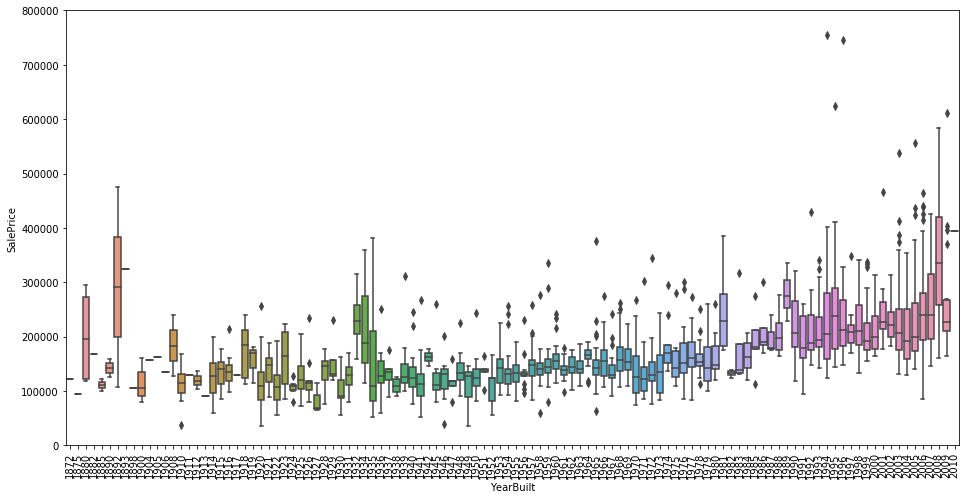
1 2 3 4 5 6 7 8 9 var = 'YearBuilt' data = pd.concat([df_train['SalePrice' ], df_train[var]], axis=1 ) f, ax = plt.subplots(figsize=(16 , 8 )) fig = sns.boxplot(x=var, y='SalePrice' , data=data) fig.axis(ymin=0 , ymax=800000 ) plt.xticks(rotation=90 )
(array([  0,   1,   2,   3,   4,   5,   6,   7,   8,   9,  10,  11,  12,
         13,  14,  15,  16,  17,  18,  19,  20,  21,  22,  23,  24,  25,
         26,  27,  28,  29,  30,  31,  32,  33,  34,  35,  36,  37,  38,
         39,  40,  41,  42,  43,  44,  45,  46,  47,  48,  49,  50,  51,
         52,  53,  54,  55,  56,  57,  58,  59,  60,  61,  62,  63,  64,
         65,  66,  67,  68,  69,  70,  71,  72,  73,  74,  75,  76,  77,
         78,  79,  80,  81,  82,  83,  84,  85,  86,  87,  88,  89,  90,
         91,  92,  93,  94,  95,  96,  97,  98,  99, 100, 101, 102, 103,
        104, 105, 106, 107, 108, 109, 110, 111]),
 <a list of 112 Text xticklabel objects>)
不知“SalePrice”是否已剔除通胀影响的价格,无法对不同建造年份的房屋价格进行比较。
1 2 3 4 5 cor_m = df_train.corr() f, ax = plt.subplots(figsize=(12 , 9 )) sns.heatmap(cor_m, vmax=.8 , square=True )
<matplotlib.axes._subplots.AxesSubplot at 0x16f6f3a2da0>
颜色越浅,表明正相关性越强
'TotalBsmtSF’和’1stFlrSF’的正相关性很强(很显然)
'GarageCars’和’GarageArea’的正相关性很强(也很显然)
上述两组正相关性很强的变量,导致数据存在多重共线性
考虑剔除其中一个变量,因为正相关性强的两个变量包含的信息是相似的
看‘SalePrice’那一列,也可以通过热力图的颜色深浅,直观地发现与‘SalePrice’正相关性较强的变量,如‘OverallQual’、‘GriLivArea’
其中:
1stFlrSF: First Floor square feet
TotalBsmtSF: Total square feet of basement area
GarageCars: Size of garage in car capacity
GarageArea: Size of garage in square feet
1 2 3 4 5 6 7 8 9 10 11 k = 10 cols = cor_m.nlargest(k, 'SalePrice' )['SalePrice' ].index cm = np.corrcoef(df_train[cols].values.T) sns.set (font_scale=1.25 ) hm = sns.heatmap(cm, cbar=True , annot=True , square=True , fmt='.2f' , annot_kws={'size' : 10 }, yticklabels=cols.values, xticklabels=cols.values) plt.show()
相关性较强的几对变量:
‘GarageCars’、‘GarageArea’
‘GriLivArea’、‘TotRmsAbvGrd’
‘TotalBsmtSF’、‘1stFlrSF’
考虑剔除每对中的一个
1 2 3 4 5 6 sns.set () cols = ['SalePrice' , 'OverallQual' , 'GrLivArea' , 'GarageCars' , 'TotalBsmtSF' , 'FullBath' , 'YearBuilt' ] sns.pairplot(df_train[cols], size=2.5 ) plt.show()
数据清洗
缺失
1 2 3 4 5 6 total = df_train.isnull().sum ().sort_values(ascending=False ) percent = (df_train.isnull().sum ()/df_train.isnull().count()).sort_values(ascending=False ) missing_data = pd.concat([total, percent], axis=1 , keys=['Total' , 'Percent' ]) missing_data.head(20 )
Total
Percent
PoolQC
1453
0.995205
MiscFeature
1406
0.963014
Alley
1369
0.937671
Fence
1179
0.807534
FireplaceQu
690
0.472603
LotFrontage
259
0.177397
GarageCond
81
0.055479
GarageType
81
0.055479
GarageYrBlt
81
0.055479
GarageFinish
81
0.055479
GarageQual
81
0.055479
BsmtExposure
38
0.026027
BsmtFinType2
38
0.026027
BsmtFinType1
37
0.025342
BsmtCond
37
0.025342
BsmtQual
37
0.025342
MasVnrArea
8
0.005479
MasVnrType
8
0.005479
Electrical
1
0.000685
Utilities
0
0.000000
当一个列的数据超过15%都是缺失,则应考虑删除该列
列’PoolQC’, ‘MiscFeature’, 'Alley’等的缺失比例较大,考虑删除
‘GarageX’几个列的缺失个数一样,但是缺失比例都较小
‘BsmtX’几个列的缺失个数也一样
1 2 3 4 5 df_train = df_train.drop((missing_data[missing_data['Total' ] > 1 ]).index, 1 ) df_train = df_train.drop(df_train.loc[df_train['Electrical' ].isnull()].index) df_train.isnull().sum ().max ()
0
异常点
1 2 3 4 5 6 7 8 SalePrice_scaled = StandardScaler().fit_transform(df_train['SalePrice' ][:, np.newaxis]) low_range = SalePrice_scaled[SalePrice_scaled[:, 0 ].argsort()][:10 ] high_range = SalePrice_scaled[SalePrice_scaled[:, 0 ].argsort()][-10 :] print ('Outer range (low) of the distribution:' )print (low_range)print ('\nOuter range (high) of the distribution:' )print (high_range)
Outer range (low) of the distribution:
[[-1.83820775]
 [-1.83303414]
 [-1.80044422]
 [-1.78282123]
 [-1.77400974]
 [-1.62295562]
 [-1.6166617 ]
 [-1.58519209]
 [-1.58519209]
 [-1.57269236]]

Outer range (high) of the distribution:
[[3.82758058]
 [4.0395221 ]
 [4.49473628]
 [4.70872962]
 [4.728631  ]
 [5.06034585]
 [5.42191907]
 [5.58987866]
 [7.10041987]
 [7.22629831]]
较低的10个值仅在-1.5到-1.9之间
而较高的10个值的跨度从3到7.5
要小心SalePrice标准化后值为7以上的样本点
1 2 3 4 5 6 var = 'GrLivArea' data = pd.concat([df_train['SalePrice' ], df_train[var]], axis=1 ) data.plot.scatter(x=var, y='SalePrice' , ylim=(0 , 800000 ))
'c' argument looks like a single numeric RGB or RGBA sequence, which should be avoided as value-mapping will have precedence in case its length matches with 'x' & 'y'.  Please use a 2-D array with a single row if you really want to specify the same RGB or RGBA value for all points.


<matplotlib.axes._subplots.AxesSubplot at 0x16f736e0ac8>
观察上图,可以发现右上方和右下方各有2个点较为异常。
右上方的两个点比较顺应整体趋势
而右下方的两个点并没有顺应整体趋势,考虑将其删去
1 2 df_train.sort_values(by='GrLivArea' , ascending=False )[:2 ]
Id
MSSubClass
MSZoning
LotArea
Street
LotShape
LandContour
Utilities
LotConfig
LandSlope
...
EnclosedPorch
3SsnPorch
ScreenPorch
PoolArea
MiscVal
MoSold
YrSold
SaleType
SaleCondition
SalePrice
1298
1299
60
RL
63887
Pave
IR3
Bnk
AllPub
Corner
Gtl
...
0
0
0
480
0
1
2008
New
Partial
160000
523
524
60
RL
40094
Pave
IR1
Bnk
AllPub
Inside
Gtl
...
0
0
0
0
0
10
2007
New
Partial
184750
2 rows × 63 columns
1 2 df_train = df_train.drop(df_train[df_train['Id' ] == 1299 ].index) df_train = df_train.drop(df_train[df_train['Id' ] == 523 ].index)
核心
testing for assumptions underlying the statistical bases for multivariate analysis.
正态性检验
1 2 3 sns.distplot(df_train['SalePrice' ], fit=norm) fig = plt.figure() res = stats.probplot(df_train['SalePrice' ], plot=plt)
很显然,‘SalePrice’并不服从正态分布
右偏
QQ图尾部(蓝点)与标准正态分布(红线)不一致
1 2 df_train['SalePrice' ] = np.log(df_train['SalePrice' ])
1 2 3 4 sns.distplot(df_train['SalePrice' ], fit=norm) fig = plt.figure() res = stats.probplot(df_train['SalePrice' ], plot=plt)
Perfect!
1 2 3 4 sns.distplot(df_train['GrLivArea' ], fit=norm) fig = plt.figure() res = stats.probplot(df_train['GrLivArea' ], plot=plt)
1 2 df_train['GrLivArea' ] = np.log(df_train['GrLivArea' ])
1 2 3 sns.distplot(df_train['GrLivArea' ], fit=norm) fig = plt.figure() res = stats.probplot(df_train['GrLivArea' ], plot=plt)
1 2 3 4 sns.distplot(df_train['TotalBsmtSF' ], fit=norm); fig = plt.figure() res = stats.probplot(df_train['TotalBsmtSF' ], plot=plt)
1 2 3 4 5 6 df_train['HasBsmt' ] = pd.Series(len (df_train['TotalBsmtSF' ]), index=df_train.index) df_train['HasBsmt' ] = 0 df_train.loc[df_train['TotalBsmtSF' ]>0 ,'HasBsmt' ] = 1 df_train.loc[df_train['HasBsmt' ]==1 ,'TotalBsmtSF' ] = np.log(df_train['TotalBsmtSF' ])
1 2 3 sns.distplot(df_train[df_train['TotalBsmtSF' ]>0 ]['TotalBsmtSF' ], fit=norm); fig = plt.figure() res = stats.probplot(df_train[df_train['TotalBsmtSF' ]>0 ]['TotalBsmtSF' ], plot=plt)
同方差性(同质性)
1 plt.scatter(df_train['GrLivArea' ], df_train['SalePrice' ])
<matplotlib.collections.PathCollection at 0x16f7589eba8>
未进行对数变换前,'GrLivArea’和’SalePrice’散点图呈锥形
进行对数变换后,不再呈锥形(上图)
1 plt.scatter(df_train[df_train['TotalBsmtSF' ]>0 ]['TotalBsmtSF' ], df_train[df_train['TotalBsmtSF' ]>0 ]['SalePrice' ])
<matplotlib.collections.PathCollection at 0x16f7589ebe0>
We can say that, in general, ‘SalePrice’ exhibit equal levels of variance across the range of ‘TotalBsmtSF’.
类别变量
需要将类别变量转化为哑变量(dummy)
1 df_train = pd.get_dummies(df_train)
Id
MSSubClass
LotArea
OverallQual
OverallCond
YearBuilt
YearRemodAdd
BsmtFinSF1
BsmtFinSF2
BsmtUnfSF
...
SaleType_ConLw
SaleType_New
SaleType_Oth
SaleType_WD
SaleCondition_Abnorml
SaleCondition_AdjLand
SaleCondition_Alloca
SaleCondition_Family
SaleCondition_Normal
SaleCondition_Partial
0
1
60
8450
7
5
2003
2003
706
0
150
...
0
0
0
1
0
0
0
0
1
0
1
2
20
9600
6
8
1976
1976
978
0
284
...
0
0
0
1
0
0
0
0
1
0
2
3
60
11250
7
5
2001
2002
486
0
434
...
0
0
0
1
0
0
0
0
1
0
3
4
70
9550
7
5
1915
1970
216
0
540
...
0
0
0
1
1
0
0
0
0
0
4
5
60
14260
8
5
2000
2000
655
0
490
...
0
0
0
1
0
0
0
0
1
0
5 rows × 222 columns